Summary
The XStream® HDVR® SDK supports a variety of render modes. These render modes are used to visualize the dataset in different ways. Render modes operate using either brute force or adaptive algorithms, and either parallel or perspective projections.
Brute Force vs. Adaptive Rendering Modes
In brute force renderings, the dataset is evaluated at sampling points along the ray path through the volume. The density of sampling points depends upon the zoom level for the dataset. At high zoom levels there will be at least one sample point per voxel, resulting in a highly detailed image. The lower the zoom level, the further apart the sample points will be. If the zoom level is low enough, some small anatomical structures may be missed because they are smaller than the sample point separation. Therefore, brute force modes are ideal for viewing at high zoom levels. Brute force modes are more computationally intensive because they sample more individual data points than adaptive rendering modes do, but they yield more detail. This is in part because the rendering algorithm, while computing a final high-detail image, uses tricubic interpolation to calculate the voxel values at the sample points during ray traversal. Brute force modes use trilinear interpolation when calculating interactive quality images. Because of the additional computational load of brute force renderings they should be used only with slab thicknesses of < 50 mm. All brute force render modes use a parallel projection.
Adaptive rendering modes make use of an octree data structure to accelerate rendering. Use of the octree structure allows the rendering algorithm to incorporate data from all voxels along the ray's traversal path through the dataset, without the brute force method of actually collecting sample values from every individual voxel. This enables adaptive rendering modes to render faster than brute force modes. Adaptive rendering modes use trilinear interpolation when calculating voxel values during ray traversal, which is less accurate than the tricubic interpolation used by brute force modes for final quality images. Because brute force modes are computationally intensive, adaptive modes should be used on datasets with a slab thickness of > 50 mm. Transfer function based render modes are only available when using the adaptive algorithm.
Due to performance considerations, brute force modes should not be used for slab thicknesses > 50 mm.
Parallel vs. Perspective Projection Rendering
Render modes using parallel projection utilize rays that are all parallel to each other. Therefore, all rendered objects appear to be the same distance from the current viewpoint regardless of their actual distance. Parallel rendering modes are useful for taking measurement points across the dataset, because there is a one-to-one relationship between pixels and length. That is, each pixel on the screen has the same absolute size relative to the dataset.
Render modes that use perspective projection utilize rays that are emitted from the center of the current viewpoint, and more closely simulate how the human visual systems works. Objects in a perspective projection appear smaller the farther they are from the camera, whereas objects appear larger the closer they are to the camera. Perspective rendering allows the viewer to explore complex regions close to or inside the dataset, and is useful for fly-through or auto-navigation of the colon, vessels, airway and nerve canals.
Parallel Projection |
Perspective Projection |
Render modes are selected by setting the RENDER_PARAMS::RenderType member to a value from the ENUM_RENDER_TYPE enumeration. Multiple values from ENUM_RENDER_TYPE may map to the same render mode. For more information on use of the RENDER_PARAMS structure, see the Render Parameters section. The appropriate ENUM_RENDER_TYPE value for each mode is shown below.
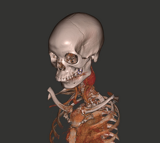
Transfer Function based rendering modes produce colored 3D volume renderings with translucent, transparent and opaque effects. The transfer function maps a voxel's Hounsfield value (or other dataset unit) to three components: color, lighting and opacity values. When rays are cast through the volume, they are differentially absorbed and colored by the voxels through which they pass, based on these three components. The result is a colored 3D volume rendering. The XStream HDVR SDK supports multiple transfer functions, allowing groups of voxels to be assigned to different transfer functions. These voxel groups can be visualized separately through the use of segmentation techniques.
Transfer Function rendering is available in the following modes.
Parallel adaptive: RT_PARALLEL
Perspective adaptive: RT_PERSPECTIVE
Maximum Intensity Projection (MIP)
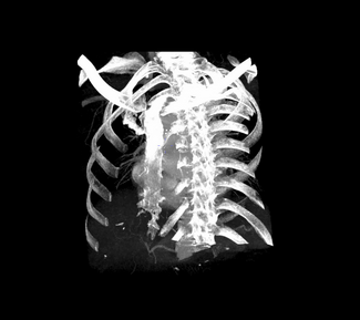
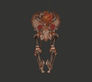
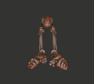
A MIP rendering is one that displays only the voxel with the highest Hounsfield value (or other dataset unit) along the ray's direction of travel. The voxel is visualized as a grayscale pixel ranging from black (minimum density) to white (maximum density). This mode is useful for identifying regions of high density, regardless of the structure's position within the dataset. This mode is best suited to visualize bone, contrast-enhanced or other materials with a high attenuation value.
MIP rendering is available in the following modes.
Parallel brute force: RT_BRUTE_FORCE_MIP or RT_THIN_MIP
Parallel adaptive: RT_THICK_MIP or RT_MIP
Perspective adaptive: RT_THICK_MIP_PERSPECTIVE
A Faded MIP rendering is similar to MIP. However, in Faded MIP voxels become darker as they increase in distance from the camera. In a conventional MIP rendering, the voxel with the highest Hounsfield value (or other dataset unit) along the ray path is always displayed. This can cause foreground structures of lower density to become obscured by background structures of high density. Use of Faded MIP rendering allows better visualization of foreground structures in these cases.
Faded MIP rendering is available in the following modes.
Parallel brute force: RT_BRUTE_FORCE_FMIP or RT_THIN_FMIP
Parallel adaptive: RT_THICK_FADED_MIP or RT_XRAY
Minimum Intensity Projection (MinIP)
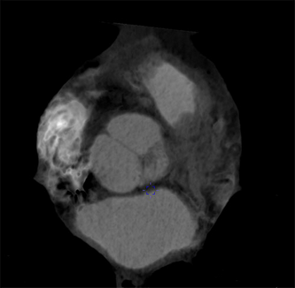
A MinIP rendering is a form of MPR rendering in which only the voxels of lowest Hounsfield value (or other dataset unit) are visualized. A MinIP image is calculated in the same manner as an MPR rendering, but the visualized image shows only voxels of minimum attenuation. MinIP images are useful for identifying regions of low relative density.
MinIP rendering is available in the following modes.
Parallel brute force: RT_BRUTE_FORCE_MINIP or RT_THIN_MINIP
Parallel adaptive: RT_THICK_MINIP
Perspective adaptive: RT_THICK_MINIP_PERSPECTIVE
Multiplanar Reconstruction (MPR-Average)
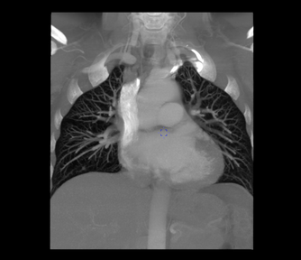
An MPR rendering is a grayscale image consisting of rendered pixels that represent the average Hounsfield value (or other dataset unit) of the voxels through which the ray passes. An MPR rendering is generated by casting rays through the volume, accumulating the value of the voxels, calculating the average value of the voxels and projecting the image onto a 2D plane. Brighter pixels correspond to material of high density, and darker pixels correspond to material of low density. MPR-Average modes work best on datasets with slab thicknesses of < 50 mm. As slab thickness increases, the image will blur more due to the averaging that takes place along the ray's traversal through the dataset.
MPR rendering is available in the following mode.
Parallel brute force: RT_BRUTE_FORCE_AVE or RT_THIN_AVE
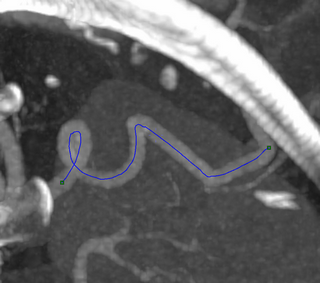
Curved Multiplanar Reformatting (Curved MPR)
Curved MPR is a special render mode that can only be used in conjunction with the Curved MPR feature. This mode must be set prior to using Curved MPR. The Curved MPR technique is used to apply a transformation to the visualization of the dataset, generally for straightening the visualization of a curved structure to improve diagnostic imaging.
Trace of a curved vessel |
Vessel straightened with CurvedMPR |
Curved MPR rendering is available in the following mode.
Non-linear brute force: RT_MPR_CURVED